Getting Started
Here is a quick-start guide for people familiar with ADI and experience using tools like VIP or pyKLIP. For installation and setup information, see the Installation and Setup section.
Expected Data Formats
ADI Cube
For standard ADI data, we store the values in a 3-dimensional array, where the first two dimensions are spatial and the third is temporal. This is how most ADI data are stored on disk (typically in FITS files) and allow specifying operations like a tensor. This cube should already be registered with the star in the center of the frames (note the center is only well-defined for odd-sized frames, even though even-sized frames will work fine).
Parallactic Angles
The parallactic angles should be stored as degrees in a vector. The parallactic angle X[i] will result in rotating frame i X[i] degrees counter-clockwise.
SDI Cube/Tensor
For standard SDI data, we store the values in a 4-dimensional array, where the first two dimensions are spatial, the third is spectral, and the fourth is temporal. This is how some SDI data are stored on disk (typically in FITS files) and allow specifying operations like a tensor. For SDI data that is stored with the temporal axis first, the dimensions should be permuted before processing (see permutedims). This cube should also be registered with the star in the center of the frame.
In addition to the SDI tensor and parallactic angles, the list of wavelengths are required (for scaling speckles) and a spectral template can be used. To create a scale list from the wavelengths or a template, use scale_list.
Algorithms
The following algorithms are implemented:
Processing Patterns
Full Frame ADI Reduction
Given an algorithm alg, we can fully process ADI data by calling alg like a function, or using the process method
julia> using ADI

julia> alg = PCA(ncomps=5)

julia> resid = alg(cube, angles)

julia> resid === process(alg, cube, angles)
true
Full Frame RDI Reduction
The only difference here is the inclusion of a reference cube.
julia> alg = PCA(ncomps=5)

julia> resid = alg(cube, angles; ref=cube_ref)
Reduction Process
The process for producing the flat, residual frame follows this general workflow
- Create a cube of the speckle approximation,
S - Subtract
Sfrom the data cube to create the residual cubeR - Derotate
Rframe-by-frame according to the parallactic angle - Collapse the derotated
R
In ADI.jl this process looks like this:
cube, angles = # load data
S = reconstruct(PCA(10), cube)
R = cube .- S
R_derotate = derotate(R, angles)
resid = collapse(R_derotate)

# or, more succinctly
R = subtract(PCA(10), cube)
resid = collapse(R, angles)
Notice how the only part of this specific to the algorithm is reconstruct? This lets us have the super-compact functional form from above without having to copy the common code for each algorithm.
Altering the Geometry
HCIToolbox.jl has utilities for geometrically filtering the input data, such as only taking an annulus of the input cube or iterating over many annuli. This is exactly the purpose of AnnulusView and MultiAnnulusView, which use indexing tricks to retrieve the pixels only within the spatial region of interest without having to copy the input data.
If you wrap a cube in one of these views, ADI.jl will handle it automatically (if the algorithm supports it). Since these views filter the pixels, the runtime performance will generally be faster than the full-frame equivalents.
ann = AnnulusView(cube; inner=15, outer=25)
res = PCA(10)(ann, angles)
# annuli of width 5 starting at 5 pixels and ending at the edge of the cube
anns = MultiAnnulusView(cube, 5; inner=5)
res = PCA(10)(anns, angles)
# use different algorithms for each annulus
N_ann = length(anns.indices)
algs = [PCA(10), PCA(9), PCA(8), ...]
res = process(algs, anns, angles)Comparison to VIP
ADI.jl took a lot of ideas from VIP and expanded them using the power of Julia. To begin with, Julia typically has smaller and more self-contained packages, so most of the basic image-processing that is used here is actually written in the HCIToolbox.jl package. In the future, I have plans to incorporate forward-modeling distributions in Firefly.jl, which currently is an active research project.
Some technical distinctions to VIP
- Julia is 1-indexed. This means all the positions for apertures, bounds, images, etc. start at 1. This is distinct from 0-based indexing in python, but is equivalent to the indexing in DS9 and IRAF.
- Julia is column-major. This means all data, when loaded from disk, will appear "transposed" from what is loaded by
astropy.io.fits. - Julia's
stduses the sample statistic (n-1degrees of freedom) while numpy'sstduses the population statistic (ndegrees of freedom). This may cause very slight differences in measurements that rely on this. - Aperture mapping - many of the
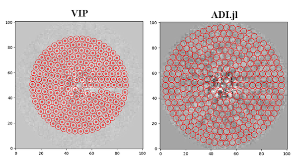
Metricsare derived by measuring statistics in an annulus of apertures. In VIP, this ring is not equally distributed- the angle between apertures is based on the exact number of apertures rather than the integral number of apertures that are actually measured. In ADI.jl the angle between apertures is evenly distributed. The same number of pixels are discarded in both packages, but in VIP they all end up in the same region of the image (see this figure). - Collapsing - by default VIP collapses a cube by derotating it then finding the median frame. In ADI.jl, the default collapse method is a weighted sum using the inverse of the temporal variance for weighting. This is documented in
HCIToolbox.collapseand can be overridden by passing the keyword argumentmethod=medianor whichever statistical function you want to use. - Image interpolation - by default VIP uses a
lanczos4interpolator from opencv, by default ADI.jl uses a bilinear b-spline interpolator through Interpolations.jl - Annular and framewise processing - some of the VIP algorithms allow you to go annulus-by-annulus and optionally filter the frames using parallactic angle thresholds. ADI.jl does not bake these options in using keyword arguments; instead, the geometric filtering is achieved through
AnnulusViewandMultiAnnulusView. Parallactic angle thresholds are implemented in theFramewisealgorithm wrapper. I've separated these techniques because they are fundamentally independent and because it greatly increases the composability of the algorithms.
The biggest difference, though, is Julia's multiple-dispatch system and how that allows ADI.jl to do more with less code. For example, the GreeDS algorithm was designed explicitly for PCA, but the formalism of it is more generic than that. Rather than hard-coding in PCA, the GreeDS algorithm was written generically, and Julia's multiple-dispatch allows the use of, say, NMF instead of PCA. By making the code generic and modular, ADI.jl enables rapid experimentation with different post-processing algorithms and techniques as well as minimizing the code required to implement a new algorithm and be able to fully use the ADI.jl API.
Feature comparison
Some notable libraries for HCI tasks include VIP, pyKLIP, and PynPoint. A table of the feature sets of these packages alongside ADI.jl is presented below. In general VIP offers the most diversity in algorithms and their applications, but not all algorithms are as feature-complete as the PCA implementation. VIP also contains many useful utilities for pre-processing and a pipeline framework. pyKLIP primarily uses the PCA (KLIP) algorithm, but offers many forward modeling implementations. PynPoint has a highly modular pre-processing module that is focused on pipelines.
| - | Pre. | Algs. | Techs. | D.M. | F.M. |
|---|---|---|---|---|---|
| ADI.jl | ✗ | median, LOCI, PCA, NMF, fixed-point GreeDS | Full-frame ADI/RDI, SDI (experimental), annular ADI* | detection maps, STIM, SLIMask, contrast curve | ✗ |
| VIP | ✓ | median, LOCI, PCA, NMF, LLSG, ANDROMEDA, pairwise frame differencing | Full-frame ADI/RDI, SDI, annular ADI/RDI* | detection maps, blob detection, STIM, ROC, contrast curve | NegFC |
| pyKLIP | ✗ | PCA, NMF, weighted PCA | Full-frame ADI/RDI, SDI, annular ADI/RDI | detection maps, blob detection, contrast curve, cross-correlation | KLIP-FM, Planet Evidence, matched filter (FMMF), spectrum fitting, DiskFM |
| PynPoint | ✓ | median, PCA | Full-frame ADI/RDI, SDI | detection maps, contrast curve | ✗ |
Column labels: Pre-processing, Algorithms, Techniques, Detection Metrics, Forward Modeling.
Techniques marked with * indicate partial support, meaning that not all algorithms are supported.